How to Look at Differences Between Three Groups on a Continuous Variable

In response to some of the discussion that inspired yesterday's post, Gary McClelland writes:

I remain convinced that discretizing a continuous variable, especially for multiple regression, is the road to perdition.

Here I explain my concerns. First, I don't buy the motivation that discretized analyses are easier to explain to lay citizens and the press. Second, I believe there is an error in your logic for computing the relative efficiency for splitting into three groups. Third, and most importantly, dichotomizing or trichotomizing two or more continuous variables in a multiple regression is an especially bad idea. In such cases, the loss of efficiency is irrelevant because the discrete predictor variables have a different correlation than the continuous variables. As a consequence, the parameter estimates from the discrete analysis are biased. I'll explain all three issues in some detail.

1. I just don't buy the motivating issue—that the essence of a regression analysis can't be explained to lay people. Explaining a regression result in terms of differences between averages is fine with me, but that doesn't require a dichotomized analysis. We assume there is some true population difference between the average case in the top group (whether that be the top half, top third, top 27%, top quarter) and the average case in the bottom group. Let's call those two population means muH and muL (for high and low). Our goal is to estimate that population mean difference. We, as statisticians, have two (at least) ways to estimate that mean difference muH – muL.

a. We do the split and compute the corresponding averages ybarH and ybarL and our estimate of muH – muL is ybarH – ybarL.

b. We regress y on x, as originally measured, to obtain yhat = b0 + b1 x. then we estimate muH – muL using (b0 + b1 xbarH) – (b0 + b1 xbarL) = b1(xbarH – xbarL).

Both are unbiased estimates of muH – muL and both can be described as "our data estimates the difference between the average person in the top group in the population and the average person in the bottom group in the population is …" The only difference between the two methods is that the variance of the estimate in (a) is greater than the variance of the estimate in (b). That implies that there will be many times when the estimate in (a) is either higher or lower than the estimate in (b). Hence, the two analyses will seldom agree on the magnitude of the raw effect. That gives researchers another degree of freedom to report the estimate that better fits their argument. We should use the the more precise regression estimate (b) and explain it in terms of a mean difference between high and low groups. If we are communicating to a lay group we should give them our best estimate and that is b1(xbarH – xbarL). We don't need to explain to them how we got our estimate of muH – muL unless they ask. and even then the explanation isn't that difficult. "We compared our prediction for a person with an average score in the top group to our prediction for a person with an average score in the low group."

2. Using extreme groups in a three-way split of a single continuous predictor: The error in your mathematical analysis, I believe, is the assumption that the residual variance remains constant and is therefore the same in Eq. 4 and Eq. 5 in Gelman & Park (2008). It is easy to disprove that assumption. The residual variance is V(e) = V(Y)(1-r^2). Discretizing changes the correlation between X and Y. Furthermore, restricting the values of Y to cases that have extreme values of X will necessarily increase the V(Y). The exception is that when r = 0, V(Y) will be unchanged. Hence, your claims about the relative efficiency of extreme groups apply if and only if r = 0. In an attached Mathematica notebook (also included the pdf if you don't use Mathematica) and an attached R simulation file, I did a detailed analysis of the relative efficiency for different values of b in the model Y = b X + e. This graph summarizes my results:

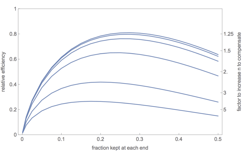
The curves represent the relative efficiency (ratio of the variances of the estimates of the slopes) for, top to bottom, slopes of b = 0, .25, 0.5, 1, 2, and 3. Given the assumption that V(e) = 1 in the full data, these correspond to correlations, respectively, of r = 0, 0.24, 0.45, 0.71, 0.89, and 0.95. The top curve corresponds to your efficiency curve for the normal distribution in your Figure 3. And, as you claim, using an extreme group split (whether the keep fraction is 0.2, 0.25, 0.27, or 0.333) is superior to a median split at all degrees of relationship between X and Y. However, relative efficiency declines as the strength of the X,Y relationship increases. Note also that the optimal fraction to keep shifts lower as the strength of the relationship increases.

Are these discrepancies important? For me and my colleagues in the social sciences, I decided the differences were of interest to geeky statisticians like you and me but probably not of practical importance. Within the range of most social science correlations (abs(r) < 0.5), the differences in the efficiency curves are trivial. And if a social scientist felt compelled for reasons of explainability to discretize the analysis, then I certainly agree that doing an extreme-groups analysis is preferable to doing a median split. However, if a researcher studying a physical industrial process (where the correlation is likely very high and high precision is desired) were tempted to do an extreme-groups analysis because it would be easier to explain to upper management, I would strongly advise against it. The relative efficiency is likely to be extremely low. On the right axis I've indexed the factor by which the sample size would need to be increased to compensate for the loss of efficiency. The price to be paid is extremely high. 3. When two or more correlated variables are analyzed via multiple regression, discretizing a continuous variable is a particularly bad idea not only because of reduced efficiency, but more importantly because discretizing changes the correlational structure of the predictors and that leads to bias in the parameter estimates. Most of the discussion in the set of median split papers in JCP concerned whether one could get away with splitting a single continuous variable which was to be analyzed in multiple regression with another continuous variable or as a covariate in an ANCOVA design. We thought both the considerable loss of power and the induced bias as a function of the predictor correlation were adequate reasons to reject such dichotomizations. I will be interested to see what your take is on that. However, I believe that doing an analysis with two discretized variables, whether by median splits or by "thirds" is a terrible idea because of the bias it induces. For median splits of two predictors with a bivariate normal distribution with correlation rho = 0.5, I can show analytically that the correlation between the dichotomized predictors will be 0.33, resulting in a confounding of the estimated slopes. Specifically, b1 = (5 b1 +b2)/6 and b2 = (b1 + 5 b2)/6. That is not good science. In the case of trichotomizing the two predictors and then using the extreme four corners of the 3 x 3 cells, I can show analytically that the predictor correlation INCREASES from 0.5 to 0.7. You can see why the correlation is enhanced in the bivariate distribution with correlation rho = 0.5 in this contour plot: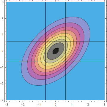

Using only the four extreme cells makes the correlation appear stronger.

I haven't yet worked through analytically the bias this will cause, but I have experimented with simulations and observed that there is an enhancement bias for the coefficients. If one coefficient is larger than the other, then the value of the larger coefficient is unbiased but the value of the smaller coefficient is increased (i've been working with all positive coefficients). For example, when predictors x and z are from a bivariate normal distribution with correlation 0.5 and the model is y = x + 2 z + e, then the cut analysis yields coefficient estimates of 1.21 and 2.05. The 21% enhancement of the smaller coefficient isn't just bad science, it isn't science at all. The source of the problem can be seen in the comparison of two tables. The first table is the predicted means using the regression equation for the full model applied to the actual cell means for x and z.

-3.7 1.2
-1.2 3.7

The following table is the mean y values for each cell (equivalently, the model derived from the cut variables).

-4.0 1.0
-1.0 4.0

In other words, the cut analysis exaggerates the differences in the cell means. This arises because the cut analysis forces a false orthogonal design. This is confounding in the same sense that bad experimental designs confound effect estimates.

A particularly disturbing example is for the model y = x + 0*z + e, the coefficients for the cut analysis are 0.96 and 0.11, a spurious effect for z. This can be seen in the table of means for the four groups:

-1.3 -1.1
1.0 1.3

In fact, the columns should have been identical as in

-1.22 -1.23
1.22 1.21

consistent with the null effect for z. This spurious effect is akin to the problem of spurious effects due to dichotomizing two variables identified by Maxwell & Delaney (1993).

In short, discretizing two continuous predictors has no place in the responsible data analyst's toolbox. At the end of section 2.8 you describe doing the appropriate full analysis as an option. I strongly disagree this is optional—it is a requirement.

You present bivariate analyses across years both for a continuous analysis (Figure 5) and an extreme-groups analysis (Figure 6). If both ways of estimating the effects were unbiased and equally efficient, we would expect the rank order of a given effect across years to remain the same as well as the rank order of the three effects for a given year to remain constant. Neither seems to be the case. The differences are not large relative to the standard error so perhaps these differences are just due to the increased variability of the discretized estimates. However, if religious attendance and income are correlated and especially if the degree of this correlation changes over the years, then I suspect that some of the differences between Figures 5 and 6 are due to bias induced by using discretized correlated predictors. I think the logits of Figure 5 transformed back to probability differences would have been more appropriate and no more difficult to explain.

I also am attaching a 5th paper in the JCP sequence—our effort at a rebuttal of their rebuttal that we posted on SSRN.

Gelman & Park (2008) argue that splitting a single continuous predictor into extreme groups and omitting the middle category produces an unbiased estimate of the difference and, although less efficient than using the continuous predictor, is less destructive than the popular median split. In this note I show that although their basic argument is essentially true, they overstate the efficiency of the extreme splits. Also their claims about optimal fractions for each distribution ignores a dependency of the optimal fraction on the magnitude of the correlation between X and Y.

In their Equations 4 and 5, Gelman & Park assume that the residual variance of Y is constant. It is easy to show that is not the case when discretizing a continuous variable, especially when using extreme groups. . . .

I don't have time to look at this right now, but let me quickly say that I prefer to model the continuous data, and I consider the discretization to just be a convenience. I'll have to look at McClelland's notes more carefully to see what's going on: is he right that we were overstating the efficiency of the comparison that uses the discretized variable? Stay tuned for updates.

P.S. I don't want to make a big deal about this, but . . . this is the way to handle it when someone says you made a mistake in a published paper: you give them a fair hearing, you don't dismiss their criticisms out of hand. And it's more than that: if you have a reputation for listening to criticism, this motivates people to make such criticisms openly. Everybody wins.

theisbefer1966.blogspot.com

Source: https://statmodeling.stat.columbia.edu/2015/11/25/gary-mcclelland-agrees-with-me-that-dichotomizing-continuous-variable-is-a-bad-idea-he-also-thinks-my-suggestion-of-dividing-a-variable-into-3-parts-is-also-a-mistake/

Share this post